# URL containing 10-minute interval weather data from Tokyo site on March 9, 2024
# Can be replaced with 10-minute data from any 's1' type observation site
jma_URL = 'https://www.data.jma.go.jp/stats/etrn/view/10min_s1.php?prec_no=44&block_no=47662&year=2024&month=3&day=9&view='Data Scraping and Parsing Weather Records from the Japan Meteorological Agency (JMA) Website Using Python
(A) Data Collection
(B) Data Preprocessing
weather data
Japan Meteorological Agency
data scraping
data parsing
library - requests
library - bs4
library - datetime
library - pytz
library - pandas
Step-by-step tutorial on scraping and parsing 10-minute weather records from the Japan Meteorological Agency (JMA) website and preparing them for further analysis using Python.

1 Introduction
The Japan Meteorological Agency (JMA) monitors and records various weather data including rainfall, wind speed and direction, temperature and relative humidity from over 840 sites across Japan through their Automated Meteorological Data Acquisition System (AMeDAS)1. Much of this data are publicly available online, and some datasets can be downloaded as CSV files. However, learning to scrape and parse weather data directly from their website with Python is useful because:
- Not all JMA datasets are available as CSV downloads
- Downloading hundreds of days of data from multiple weather stations manually can be painful
Data scraping allows you to retrieve any weather data available on the JMA website in a consistent and reproducible manner. Although it will require some time and effort upfront to write the code, once set up, the code can be easily modied to scrape data from different dates or weather stations.
In this tutorial, I’ll walk through a method to scrape and parse 10-minute interval weather data of the Tokyo JMA weather station using Python libraries requests and Beautiful Soup. The tabular data will be cleaned and preprocessed with headers and wind directions translated from Japanese to English, and useful details will be attributed to the timestamps using datetime and pytz libraries.
1.1 What You’ll Learn in This Tutorial
By the end of this tutorial, you’ll learn how to:
- Scrape tabular weather data from JMA’s website using
requestslibrary - Parse and give structure to the raw data with
Beautiful Souplibrary - Clean and preprocess the timestamps of the data with
datetimeandpytzlibraries - Save the data as a CSV file
If you prefer to skip the explanations and jump straight to the implementation, you can download the code from my GitHub repository.
Here is the list of things you’ll need to run the code.
1.2 Prerequisites
- A copy of either the
jma-weather-scraping.ipynbJupyter notebook orjma-weather-scraping.pyPython script from my GitHub repository data/subfolder for saving the CSV output- Python libraries
requestsbs4datetimepytzpandas
1.3 Jargon
Data scraping: Using code to extract information from a web page or a source that’s primarily designed for human viewing. In this blog post, we’ll be pulling data from an HTML table on the JMA site.
Data parsing: Converting raw or unstructured text into something structured and easy to work with. For example, turning HTML table rows into a tidy pandas DataFrame.
2 Scrape, Parse, Clean and Save Japan Weather Data
Here are the steps involved in collecting weather data from the JMA website:
- Find the URL you want to retrieve data from
- Use
requestslibrary to scrape all data on the web page - Use an HTML parser and
Beautiful Souplibrary to give structure to the raw data - Navigate the HTML to identify the table with the desired data
- Convert the desired data into a
pandasDataFrame - Attribute useful details to the timestamps using
datetimeandpytzlibraries - Save the DataFrame as a CSV file
Let’s start with step 1.
2.1 Step 1: Designate the URL with the Weather Data
First, we’ll need the URL of the JMA webpage that contains the specific data we want to scrape. If you’d like to know the actual data scraping and parsing methods and do not care much for finding a specific JMA station, skip ahead to step 2.
TipUpdate Alert!
I’ve made a user-friendly map of the weather stations in Japan. It’s an interactive and informative map that shows all the JMA weather stations, and provides you with the information needed for designating the URL. Namely, the block_no, prec_no and whether the station is an a or s type.
For those interested in finding your own JMA weather station, you can navigate the records of past weather data. Refer to Figure 1 below to:
- Narrow down on the JMA weather site by designating the prefecture (red box)
- Pinpoint the observation site within the prefecture (orange box, activated once you designate the prefecture)
- Choose the year, month and day for the desired data (green box)
- Select the type of weather data to access (blue box)
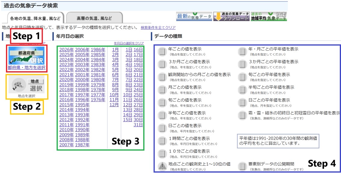
You may need a combination of Google maps, a translation app and trial and error to navigate to your desired URL. You’ll also notice that the column headers in the tables differ depending on the type of data you’ve selected from the blue box in Figure 1.
For the remainder of this blog post, we’ll work with the 10-minute interval weather records. You can select the “10分ごとの値” option located on the left column within the blue box, second from the bottom for a JMA observation site and date of your preference. I’ve provided a default test URL below, which accesses 10-minute interval weather records from the Tokyo site on March 9, 2024.
Accessing this URL, we find the tabular weather data which we will be scraping:
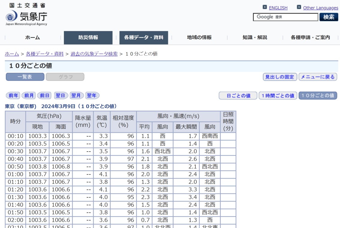
2.2 Step 2: Data Scraping with the requests Library
Next, we’d like to scrape all the HTML from the webpage. We’ll need to import the requests library to do the scraping.
# Library required for data scraping
import requests
The requests.get() function inside this library can send an HTTP GET request to the designated URL:
# HTTP GET request to jma_URL
# Execute care to avoid running multiple requests in a very short period of time
step2_resp = requests.get(jma_URL)
This returns a Response object, a class defined by the requests library, that stores the server’s reply when accessing the designated URL. The Response object has many attributes, including its content.
print("Returned object type:\n\t", type(step2_resp))

# Properties of Response object
step2_prop = step2_resp.__dict__.keys()
print("\nProperties and attributes in object:")
for prop_now in step2_prop:
    print('\t', prop_now)
Returned object type:
<class 'requests.models.Response'>
Properties and attributes in object:
_content
_content_consumed
_next
status_code
headers
raw
url
encoding
history
reason
cookies
elapsed
request
connectionSome of the other Response object attributes are useful for other applications, such as error handling. For now, we’ll ignore these and parse the HTML content with Beautiful Soup.
2.3 Step 3: Initial HTML Parsing with Beautiful Soup
With the response in hand, we can now parse the raw HTML. Import the BeautifulSoup() function from bs4:
# Import the BeautifulSoup function from bs4 library
from bs4 import BeautifulSoup
Much like how humans understand a sequence of words only when the sequence follows a set of known grammatical rules, a computer program needs to know what to expect to make sense of the raw data. In other words, when a program “reads” HTML, it needs an HTML parser to provide the rules for understanding and processing the raw HTML.
We’ll use Python’s built-in HTML parser, html.parser, to make sense of the contents of the Response object from step 2. This will return a BeautifulSoup object.
# HTML parser to make sense of the Response object
step3_soup = BeautifulSoup(step2_resp.content, "html.parser")
print("Returned object type:\n\t", type(step3_soup))
Returned object type:
<class 'bs4.BeautifulSoup'>After parsing HTML with BeautifulSoup, we can safely navigate the contents. Namely, HTML consists of tags that define specific sections within the content. Most elements follow the pattern:
<tag_name> ...content... </tag_name>Tags are often nested in a form of hierarchy. For example, every webpage can be broadly divided into two major sections, each with subsections:
<head>contains metadata, scripts, page title<body>contains the visible content, including the tabular data
Let us print just the <head> section to see what structured HTML looks like:
print(step3_soup.head.prettify())<head>
<meta charset="utf-8"/>
<title>
気象庁|過去の気象データ検索
</title>
<meta content="気象庁 Japan Meteorological Agency" name="Author"/>
<meta content="気象庁 Japan Meteorological Agency" name="keywords"/>
<meta content="気象庁|過去の気象データ検索" name="description"/>
<meta content="text/css" http-equiv="Content-Style-Type"/>
<meta content="text/javascript" http-equiv="Content-Script-Type"/>
<link href="/com/css/define.css" media="all" rel="stylesheet" type="text/css"/>
<link href="../../css/default.css" media="all" rel="stylesheet" type="text/css"/>
<script language="JavaScript" src="/com/js/jquery.js" type="text/JavaScript">
</script>
<script language="JavaScript" src="../js/jquery.tablefix.js" type="text/JavaScript">
</script>
<style media="all" type="text/css">
<!-- @import url(/com/default.css); -->
</style>
<link href="../../data/css/kako.css" media="all" rel="stylesheet" type="text/css"/>
<link href="../../data/css/print.css" media="print" rel="stylesheet" type="text/css"/>
</head>
The nested hierarchy structure can be easily spotted in the first lines:
<head>
  ...
  <title>
  気象庁|過去の気象データ検索
  </title>
  ...
</head>
In a similar manner, the tabular data to extract is contained within <body> ...tabular data... </body>.
2.4 Step 4: Identify the Target Table
Unfortunately, the HTML body contains much more than the tabular data. If you are curious as to just how much content is inside the HTML body, try running the following code on your own:
print(step3_soup.body)You can scroll through the whole HTML and manually search out the tags and identifiers associated with the desired tabular data. However, I will show you two slightly more sophisticated 🧐 search methods: a top-down and a bottom-up approach. The former requires some manual clicking, while the latter is more code-based.
2.4.1 Step 4-A: Top-Down Approach to Locating the Target Table
You can inspect the HTML code of the JMA website manually and find table attributes with the top-down approach. First, access the URL you are scraping data from, and right-click on the website and select “Inspect”. Your screen should split in half vertically, much like Figure 3. Hover over the main table containing the weather data, which should become highlighted in blue. The top right corner will show the HTML code corresponding to the tabular data.
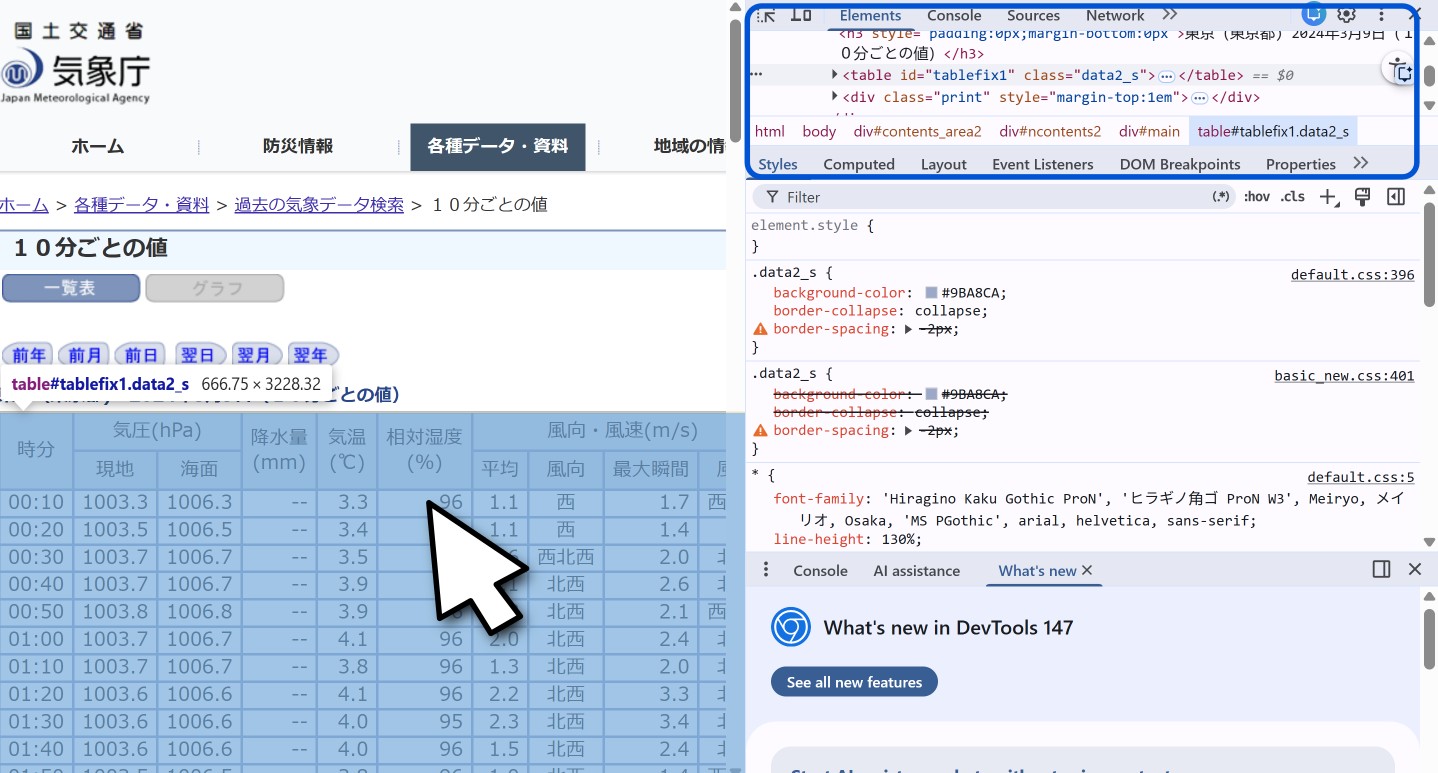
A closer view of the the HTML code in Figure 4 shows that we have <table> tags with a specific id and class. Specifically, the desired table has:
- ID of
tablefix1 - class of
data2_s
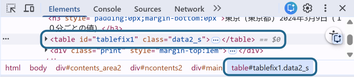
This approach allows us to pinpoint the target table from a top-down approach. However, we can also find the table using a bottom-up approach.
2.4.2 Step 4-B: Bottom-Up Approach to Locating the Desired Table
The bottom-up approach to locating the desired table takes advantage of the following:
- Target data is likely within
<table> ... </table>tags - Target data contains
'00:10'as a data element as seen in Figure 2
The BeautifulSoup.find_all() method can search for all <table> tags.
# Find all the <table> tags
step4_tables = step3_soup.body.find_all('table')

print("Total number of <table> tags:\t", len(step4_tables), '\n')
Total number of <table> tags: 6
The bottom-up coding based method reveals that the URL we were accessing contains 6 tables. We can pinpoint the desired table by searching for the table containing '00:10' as a string.
# Search for '00:10' string in the table
for table in step4_tables:
    print(table.attrs) # Print attributes of the table

    # If the '00:10' string is inside this table
    if table.find_all(string='00:10') != []:
        step4_id = table.attrs['id']
        step4_class = table.attrs['class'][0]
        print('\tFound the target table with ID', step4_id, 'and class', step4_class)
        # If the table contains the '00:10' string, print out the first five rows
        table_contents = table.find_all('tr')
        for i in range(3):
            print('\t\t', table_contents[i])
{'style': 'float:left'}
{'style': 'margin-left: auto'}
{'style': 'float:left;margin-top: 25px'}
{'style': 'margin-left: auto;margin-top: 25px'}
{'id': 'tablefix1', 'class': ['data2_s']}
Found the target table with ID tablefix1 and class data2_s
<tr class="mtx"><th rowspan="2" scope="col">時分</th><th colspan="2" scope="colgroup">気圧(hPa)</th><th rowspan="2" scope="col">降水量<br/>(mm)</th><th rowspan="2" scope="col">気温<br/>(℃)</th><th rowspan="2" scope="col">相対湿度<br/>(%)</th><th colspan="4" scope="colgroup">風向・風速(m/s)</th><th rowspan="2" scope="col">日照<br/>時間<br/>(分)</th></tr>
<tr class="mtx" scope="col"><th scope="col">現地</th><th scope="col">海面</th><th scope="col">平均</th><th scope="col">風向</th><th scope="col">最大瞬間</th><th scope="col">風向</th></tr>
<tr class="mtx" style="text-align:right;"><td style="white-space:nowrap">00:10</td><td class="data_0_0">1003.3</td><td class="data_0_0">1006.3</td><td class="data_0_0">--</td><td class="data_0_0">3.3</td><td class="data_0_0">96</td><td class="data_0_0">1.1</td><td class="data_0_0" style="text-align:center">西</td><td class="data_0_0">1.7</td><td class="data_0_0" style="text-align:center">西南西</td><td class="data_0_0"></td></tr>
{'style': 'margin-left:auto;margin-right:0px'}By selectively searching for the '00:10' string nested inside <table> tags, we have successfully isolated the meteorological data buried inside the long HTML <body>. The contents within the first few table rows (as specificed by <tr> tags) confirm that the desired data is, indeed, in this table.
As with the top-down approach, we have successfully pinpointed the desired table attributes as:
- ID of
tablefix1 - class of
data2_s
2.5 Step 5: Extract the Desired Table by Rows
We can select the one desired table by specifying either #id or .class in the soup.select() method:
# Select the target table with the table id
table_id = 'table#' + step4_id
step5_targetTable = step3_soup.select(table_id)

# Alternate method using table class instead of id
#table_class = 'table.' + step4_class
#step5_targetTable = step3_soup.select(table_class) # Alternative method

print("Number of tables selected:\t", len(step5_targetTable))
Number of tables selected: 1However, this single extracted table is still in HTML format. HTML with tags are difficult to use as is in data analysis projects. For the tabular data to be useful, we need to extract the data in each table cell and reformat it into a pandas DataFrame.
To restructure the data format, we will rewrite the soup.select() function to search for table rows, or <tr> tags, instead of the <table> tags.
# Select all rows within the target table
step5_tableRows = step3_soup.select('table#' + step4_id + ' tr')
This provides us with an object with 146 separate table rows. Inspecting the first few confirms we’ve successfully isolated the data we need.
print("Number of rows in table:\t", len(step5_tableRows))

# Print out the first couple table rows
for i in range(3):
    print('\t', step5_tableRows[i])
Number of rows in table: 146
<tr class="mtx"><th rowspan="2" scope="col">時分</th><th colspan="2" scope="colgroup">気圧(hPa)</th><th rowspan="2" scope="col">降水量<br/>(mm)</th><th rowspan="2" scope="col">気温<br/>(℃)</th><th rowspan="2" scope="col">相対湿度<br/>(%)</th><th colspan="4" scope="colgroup">風向・風速(m/s)</th><th rowspan="2" scope="col">日照<br/>時間<br/>(分)</th></tr>
<tr class="mtx" scope="col"><th scope="col">現地</th><th scope="col">海面</th><th scope="col">平均</th><th scope="col">風向</th><th scope="col">最大瞬間</th><th scope="col">風向</th></tr>
<tr class="mtx" style="text-align:right;"><td style="white-space:nowrap">00:10</td><td class="data_0_0">1003.3</td><td class="data_0_0">1006.3</td><td class="data_0_0">--</td><td class="data_0_0">3.3</td><td class="data_0_0">96</td><td class="data_0_0">1.1</td><td class="data_0_0" style="text-align:center">西</td><td class="data_0_0">1.7</td><td class="data_0_0" style="text-align:center">西南西</td><td class="data_0_0"></td></tr>With the desired table extracted in rows, we can now clean and preprocess the data to store it as a pandas DataFrame.
2.6 Step 6: Clean the Data and Prepare a DataFrame Using for Loops
From the isolated table rows, we extract and clean the weather data and place them into a structured pandas DataFrame using a for loop to work through each row.
Referring back to the sample table rows from the previous step, a few things stand out:
- The first two table rows contain no data, only headers
- Every data row begins with a
<td>or table data tag containing the time in'HH:MM'format - All remaining meteorological values appear inside
<td class="data_0_0">elements.
We can use these patterns to guide our parsing when working row-by-row in the for loop.
At the same time, we identify three potential issues with the data:
- Issue 1: The headers are in Japanese and need to be translated into English
- Issue 2: Wind direction is also in Japanese
- Issue 3: The timestamps of each data row is
'HH:MM'which can be risky when the data becomes detached from the date information
We’ll incorporate these data preprocessing steps in the for loop as well.
But first, we’ll, import the pandas library.
# Import the pandas library to deal with dataframes
import pandas as pd
Then, create an empty DataFrame. I’ve provided the English translation of the column headers below which resolves the first issue.
# The Tokyo observation site (type s1) has 11 columns of data
headers_s1 = (['time',
               'local atmospheric pressure (hPa)',
               'sea level pressure (hPa)',
               'precipitation (mm)',
               'temperature (℃)',
               'relative humidity',
               'average wind speed (m/s)',
               'average wind direction',
               'max wind speed (m/s)',
               'max wind direction',
               'sunshine (minutes)'])

# If you are using a 'a1' type observation site, use the headers below
headers_a1 = (['time',
               'precipitation (mm)',
               'temperature (℃)',
               'relative humidity',
               'average wind speed (m/s)',
               'average wind direction',
               'max wind speed (m/s)',
               'max wind direction',
               'sunshine (minutes)'])

# Specify the header you'll be using
headers_now = headers_s1 # Change to headers_a1 if using 'a1' type observation site

# Empty dataframe to fill with data
step6_df = pd.DataFrame(columns=headers_now)
Here are the steps involved in the for loop to simultaneously extract and clean the weather data:
- Skip the first two table rows which contain only headers and no numerical data
- Extract the first data, corresponding to the timestamps written as
'HH:MM' - Convert timestamps into datetime objects to make it clear
- Attribute time zone information to timestamps to make it unmistakable
- Extract the remaining meteorological values with the
<td class="data_0_0">elements- For wind direction data, translate the Japanese wind direction into English before storing it into the DataFrame.
Start by skipping the header information.
2.6.1 Step 6-1: Skip Rows Corresponding to Column Headers
We’ll filter out the rows containing just the column headers. These are characterized by rows that do not contain any data_0_0 class data. As such, the method call of soup.select('td.data_0_0') will return an empty list. This will safely skip the column headers table rows, regardless of the number of rows the original table contains.
# Iterate through each row in the table
for rowNow in step5_tableRows:
    # Search for the data_0_0 class (actual weather data)
    list_data = rowNow.select('td.data_0_0')

    if len(list_data) == 0:
        # There is no data in this row (ie. column headers), so skip
        print("Skipping row: ", rowNow)
        continue
Skipping row: <tr class="mtx"><th rowspan="2" scope="col">時分</th><th colspan="2" scope="colgroup">気圧(hPa)</th><th rowspan="2" scope="col">降水量<br/>(mm)</th><th rowspan="2" scope="col">気温<br/>(℃)</th><th rowspan="2" scope="col">相対湿度<br/>(%)</th><th colspan="4" scope="colgroup">風向・風速(m/s)</th><th rowspan="2" scope="col">日照<br/>時間<br/>(分)</th></tr>
Skipping row: <tr class="mtx" scope="col"><th scope="col">現地</th><th scope="col">海面</th><th scope="col">平均</th><th scope="col">風向</th><th scope="col">最大瞬間</th><th scope="col">風向</th></tr>Once the column headers are skipped, we’d like to extract the first data element in the row.
2.6.2 Step 6-2: Extract the Timestamps
After skipping the rows with no data, we’ll extract the first data, which are timestamps when the weather data were collected. Since the first <td> tag in each valid row always contains the timestamp, we can
- Use
soup.select_one('td')to pull out just the first element - Clean the timestamp string with
.text.strip()- Remove HTML tags with
.text() - Remove extra spaces with
.strip()
- Remove HTML tags with
- Assign it to the first column of the DataFrame using
df.loc[]attribute
Let’s add this code to the for loop from before:
# Iterate through each row in the table
rowCount = 0
for rowNow in step5_tableRows:
    # Search for the data_0_0 class that contains the weather data
    list_data = rowNow.select('.data_0_0')

    if len(list_data) == 0:
        # There is no data in this row (ie. it is a column headers), so skip
        #print("Skipping row: ", rowNow)
        continue

    else:
        # Extract time
        time1 = rowNow.select_one('td') # Select just the first <td> tag element
        time2 = time1.text.strip()      # Remove the tags with .text(). Remove extra spaces with strip()
        #print(time2)

        # Assign the time to the first column in the DataFrame
        step6_df.loc[rowCount, headers_now[0]] = time2

        # Increment rowCount
        rowCount = rowCount + 1
You can verify that all timestamps from '00:10' to '24:00' have been assigned to the DataFrame by inspecting the first and last time entries:
print("First few lines:")
print(step6_df['time'].head())
print("\nLast few lines:")
print(step6_df['time'].tail())
First few lines:
0 00:10
1 00:20
2 00:30
3 00:40
4 00:50
Name: time, dtype: object
Last few lines:
139 23:20
140 23:30
141 23:40
142 23:50
143 24:00
Name: time, dtype: objectThe timestamp format of 'HH:MM' can get quickly confusing once we start processing data across multiple days. Even if the date information is stored in the CSV filenames, once in the workspace, timestamps can become easily detached from its date information.
The simple solution is to convert the 'HH:MM' timestamps into a more informative 'yyyy-mm-dd HH:MM' notation. However, if we decide to combine data from several sources, we may have to deal with data from different time zones. In such cases, even the 'yyyy-mm-dd HH:MM' notation becomes insufficient.
To make the timestamps self-evident, we can add two more attributes.
- Use datetime type objects to store the timestamps as
'yyyy-mm-dd HH:MM' - Incorporate time zones to datetime objects
2.6.3 Step 6-3: Convert Timestamps to datetime Objects
Currently, timestamps are stored as strings:
# Check the type of the timestamps
pickedTime = step6_df.loc[4, 'time']
pTime_type = type(pickedTime)
print(pickedTime, "\ttype: ", pTime_type)
00:50 type: <class 'str'>To manage datetime objects, we need to import the datetime module:
# Import datetime library
import datetime as dt
The datetime object inside the datetime library can explicitly store year, month, day, hour, and minute information, making it unmistakable. They can be created manually using the dt.datetime() function:
# Check what a typical datetime object looks like
pickedTime_dt = dt.datetime(2024, 3, 9, 0, 50)# March 9, 2024, 0:50
pTime_dt_type = type(pickedTime_dt)
print(pickedTime_dt, "\ttype: ", pTime_dt_type)
2024-03-09 00:50:00 type: <class 'datetime.datetime'>We use the same idea, converting the timestamp string into a datetime object inside our row-by-row parsing workflow. To recreate the complete timestamp, we use:
- A known date, provided by the user as a tuple like (2024, 3, 9)
- The timestamp string extracted from the first
<td>element in each row
Python’s datetime.strptime() function can easily convert timestamp strings like '00:50' into appropriate hour and minute values.
Below is the updated parsing loop with datetime handling added:
# test date specified by user
test_date = (2024, 3, 9)

# Iterate through each row in the table
rowCount = 0
for rowNow in step5_tableRows:
    # Search for the data_0_0 class that contains the weather data
    list_data = rowNow.select('.data_0_0')

    if len(list_data) == 0:
        # There is no data in this row (ie. it is a column headers), so skip
        #print("Skipping row: ", rowNow)
        continue

    else:
        # Convert time from string to datetime object
        # Split up target_date tuple into year, month and day
        target_year = test_date[0]
        target_month = test_date[1]
        target_day = test_date[2]

        # Extract time
        time1 = rowNow.select_one('td') # Select just the first <td> tag element
        time2 = time1.text.strip()      # Remove the tags with .text(). Remove extra spaces with strip()
        #print(time2)

        # The last timestamp may be 0:00 for the next day, which may cross over into next month or even year
        if (time2 == '24:00'):
            # Set output_datetime as 23:59 of the current day, then add one minute.
            # This should deal with changes in the day, month or even the year
            deltaTime = dt.timedelta(minutes=1)
            dateTimeNow = dt.datetime(target_year, target_month, target_day, 23, 59) + deltaTime

        else:
            # Otherwise, extract the hour and minutes and use that as the hour and minute
            time3 = dt.datetime.strptime(time2, '%H:%M')
            dateTimeNow = dt.datetime(target_year, target_month, target_day, time3.hour, time3.minute)

        # Assign the time to the first column in the DataFrame
        step6_df.loc[rowCount, headers_now[0]] = dateTimeNow

        # Increment rowCount
        rowCount = rowCount + 1
As the JMA weather data collected every 10 minutes for a given day starts from '00:10', and ends with '24:00', we’ve installed an if-else statement to deal with the unconventional '24:00' timestamp.
Checking the type of the timestamp confirms that we are now dealing with datetime type objects.
# Check how the timestamps look as datetime objects
pickedTime = step6_df.loc[4, 'time']
pTime_type = type(pickedTime)
print(pickedTime, "\ttype: ", pTime_type)
2024-03-09 00:50:00 type: <class 'datetime.datetime'>2.6.4 Step 6-4: Attribute Time Zones to Timestamps
The datetime object created in the previous step is almost complete, but not quite. When combining information from multiple sources, it is beneficial to attach a time zone.
Specifically, JMA weather data is (logically) recorded in Japan Standard Time (JST). However, if you decide to download and analyze your Fitbit data, these are recorded in UTC (Coordinated Universal Time).
If you try to combine these without explicit time zone information, you’ll quickly run into alignment problems, shifting timestamps, and subtle bugs.
To work with time zones in Python, we’ll use the pytz library.
# Import the pytz library to deal with time zones
import pytz
Then, use pytz.timezone() to specify the appropriate time zone for the data. In our case, we’ll be using the time zone in Tokyo:
# Specify the time zone for Japan
JMA_tz = pytz.timezone('Asia/Tokyo') # Create a time zone in Japan time
Time zones are attached to a datetime object using the localize() method:
# Check what a typical time zone-aware datetime object looks like
pickedTime_dt_tz = JMA_tz.localize(dt.datetime(2024, 3, 9, 0, 50)) # 0:50 on March 9, 2024
pTime_dt_tz_type = type(pickedTime_dt_tz)
print(pickedTime_dt_tz, "\ttype: ", pTime_dt_tz_type) # datetime object now has a time zone
2024-03-09 00:50:00+09:00 type: <class 'datetime.datetime'>You’ll notice that datetime objects created with this method now has +09:00 appended to it. This indicates that Japan is nine hours ahead of Coordinated Universal Time (UTC).
We can now apply this idea to the timestamps extracted from the HTML table within the for loop. However, instead of handling time parsing inside the main scraping loop (as we did earlier), we’ll make our code cleaner and modular by creating a helper function, ConvertDateTime().
This function:
- Takes a row of the HTML
<table> - Extracts the timestamp string (e.g.,
'00:50') - Converts it into a datetime object using the user-specified date
- Attaches the correct time zone
- Handles special cases like
'24:00'(which belongs to the next day)
def ConvertDateTime(row_of_data, target_tz, target_date):
    """Function to take in a row of data, extract the time stamp, convert it to a datetime object in a local time zone
    AUTHOR: Mai Tanaka (www.DataDrivenMai.com)
    DATE: 2026-03-31
    REQUIRES: row_of_data = html table row where the first <td> cell contains the time in the form of %H:%M
              target_tz = target timezone as an pytz.timezone object
              target_date = (year, month , day) tuple to assign to the datetime object
    RETURNS:  output_datetime = datetime object in the specified local timezone
    """

    # Split up target_date tuple into year, month and day
    target_year = target_date[0]
    target_month = target_date[1]
    target_day = target_date[2]

    # Timestamp is the first td element in the row
    temptime = row_of_data.select_one('td')

    # Strip away the tags and excess spaces
    temptime = temptime.text.strip()

    # The last timestamp may be 0:00 for the next day, which may cross over into next month or even year
    if (temptime == '24:00'):
        # Set output_datetime as 23:59 of the current day, then add one minute.
        # This should deal with changes in the day, month or even the year
        deltaTime = dt.timedelta(minutes=1)
        tempDateTime = dt.datetime(target_year, target_month, target_day, 23, 59) + deltaTime

    else:
        # Otherwise, extract the hour and minutes and use that as the hour and minute
        temptime = dt.datetime.strptime(temptime, '%H:%M')
        tempDateTime = dt.datetime(target_year, target_month, target_day, temptime.hour, temptime.minute)

    # Attach a time zone
    output_datetime = target_tz.localize(tempDateTime)

    # Return the datetime
    return output_datetime
Incorporate ConvertDateTime() function into the for loop to make the timestamps time zone aware:
# test date specified by user
test_date = (2024, 3, 9)

# Iterate through each row in the table
rowCount = 0
for rowNow in step5_tableRows:

    # Search for the data_0_0 class that contains the weather data
    list_data = rowNow.select('.data_0_0')

    if len(list_data) == 0:
        # There is no data in this row (ie. it is a column headers), so skip
        #print("Skipping row: ", rowNow)
        continue

    else:
        # Convert time from string to datetime with time zone and assign it
        time3 = ConvertDateTime(rowNow, JMA_tz, test_date)
        step6_df.loc[rowCount, headers_now[0]] = time3

        # Increment rowCount
        rowCount = rowCount + 1
We can see that the timestamps now have a time zone attributed to it:
# Check how time zone aware timestamps look like
pickedTime_loop = step6_df.loc[4, 'time']
pTime_loop_type = type(pickedTime_loop)
print(pickedTime_loop, "\ttype: ", pTime_loop_type)
2024-03-09 00:50:00+09:00 type: <class 'datetime.datetime'>With proper time zone metadata, any downstream analysis (plotting, merging, resampling, aligning time series, etc.) will remain accurate and consistent.
Thus far in the for loop, we have omitted the column headers, extracted the timestamps and converted it into datetime objects with a time zone and transferred these values to a pandas DataFrame. All that remains is to migrate the weather data.
2.6.5 Step 6-5: Retrieve the Meteorological Data
Recall that the remaining meteorological data is associated with the data_0_0 class element. We’ll use a nested for loop that looks for <td class="data_0_0"> data element, clean the string, and insert it into the DataFrame.
Additionally, wind direction data are recorded as Japanese kanji. We will translate these into English compass notation (NESW notation) within the for loop.
I’ve provided you with the ConvertKanji2NESW() function that translates the Japanese kanji into English compass notation:
def ConvertKanji2NESW(kanji_windDir):
    """Function to convert the wind direction from kanji to English
    AUTHOR:     Mai Tanaka (www.DataDrivenMai.com)
    DATE:       2026-03-31
    REQUIRES:   kanji_windDir = Full kanji indicating wind direction (eg. '北東')
    RETURNS:    english_windDir = Wind direction in English in N/E/S/W notation (eg. 'NE')
    """
    # Start with an empty string
    english_windDir = ''

    # Handle the special case: 静穏 (tranquil or no wind)
    if kanji_windDir == '静穏':
        english_windDir = 'tranquil'
        return english_windDir

    # Kanji to character (NESW) conversion, character-by-character
    for kanji_char in kanji_windDir:
        if kanji_char == '北':
            english_windDir = english_windDir + 'N'
        if kanji_char == '東':
            english_windDir = english_windDir + 'E'
        if kanji_char == '南':
            english_windDir = english_windDir + 'S'
        if kanji_char == '西':
            english_windDir = english_windDir + 'W'

    # Return English wind direction
    return english_windDir
Working through the tabular data cell-by-cell, each weather data element is cleaned using .text() and .strip() to remove the HTML tags and spaces, respectively. If the data element corresponds to ‘wind direction’, we apply the ConvertKanji2NESW() function above. The cleaned data can finally be placed in the pandas DataFrame under the appropriate header using df.loc[].
# test date specified by user
test_date = (2024, 3, 9)

# Iterate through each row in the table
rowCount = 0
for rowNow in step5_tableRows:

    # Search for the data_0_0 class that contains the weather data
    list_data = rowNow.select('.data_0_0')

    if len(list_data) == 0:
        # There is no data in this row (ie. it is a column headers), so skip
        #print("Skipping row: ", rowNow)
        continue

    else:
        # Convert time from string to datetime with time zone and assign it
        time3 = ConvertDateTime(rowNow, JMA_tz, test_date)
        step6_df.loc[rowCount, headers_now[0]] = time3

        # Work through each data element to extract meteorological data
        columnCount = 1
        for dataNow in list_data:
            # Extract just the data (remove tags and spaces)
            justData = dataNow.text.strip()

            # If the data type is wind direction, convert from Kanji to alphabet
            if "wind direction" in headers_now[columnCount]:
                justData = ConvertKanji2NESW(justData)

            # Save the data into the appropriate location and increment columnCount
            step6_df.loc[rowCount, headers_now[columnCount]] = justData
            columnCount = columnCount + 1

        # Increment rowCount
        rowCount = rowCount + 1
A quick check of the first few lines in the resulting DataFrame confirms that all data values of time, atmospheric pressure, temperature, humidity, wind speed and others, have been successfully extracted. Furthermore, wind direction has been converted from Japanese kanji to English. Sunshine remains blank as the original HTML table did not contain any value.
# DataFrame should contain all weather data
step6_df.head()| time | local atmospheric pressure (hPa) | sea level pressure (hPa) | precipitation (mm) | temperature (℃) | relative humidity | average wind speed (m/s) | average wind direction | max wind speed (m/s) | max wind direction | sunshine (minutes) | |
|---|---|---|---|---|---|---|---|---|---|---|---|
| 0 | 2024-03-09 00:10:00+09:00 | 1003.3 | 1006.3 | -- | 3.3 | 96 | 1.1 | W | 1.7 | WSW | |
| 1 | 2024-03-09 00:20:00+09:00 | 1003.5 | 1006.5 | -- | 3.4 | 96 | 1.1 | W | 1.4 | W | |
| 2 | 2024-03-09 00:30:00+09:00 | 1003.7 | 1006.7 | -- | 3.5 | 96 | 1.6 | WNW | 2.0 | NW | |
| 3 | 2024-03-09 00:40:00+09:00 | 1003.7 | 1006.7 | -- | 3.9 | 97 | 2.1 | NW | 2.6 | NW | |
| 4 | 2024-03-09 00:50:00+09:00 | 1003.8 | 1006.8 | -- | 3.9 | 96 | 1.8 | NW | 2.1 | WNW |
The final step is to save the pandas DataFrame as a CSV for use in subsequent data analysis projects.
2.7 Step 7: Save DataFrame as a CSV File
In the final step, we save the fully populated and cleaned DataFrame as a CSV file. We can use pandas’ built-in pandas.to_csv() method to write the data out. Just specify the desired file path (and make sure the directory exists in your local environment), disable the index column, and choose an appropriate text encoding (UTF-8 is a safe default).
# Specify a strong filename in a directory that exists
fileName = 'jma_weather_scraping_jupyter.csv'
dirName = 'data/'
savefileName = dirName + fileName
step6_df.to_csv(savefileName, index=False, encoding='utf-8')
However, when you load this file back in with a plain pd.read_csv(), the timestamps looks like datetime objects, but are actually just strings:
# Load the dataframe in the most basic manner
step7_df1 = pd.read_csv(savefileName)

# Check the type of the timestamps after loading
pickedTime_load = step7_df1.loc[4, 'time']
pTime_load_type = type(pickedTime_load)
print(pickedTime_load, "\ttype: ", pTime_load_type)
2024-03-09 00:50:00+09:00 type: <class 'str'>To ensure pandas correctly interprets the date column as datetime objects, include the parse_dates argument when reading the file. In most cases, simply listing the column name is enough:
# Load the dataframe with parse_dates
step7_df2 = pd.read_csv(savefileName, parse_dates=['time'])

# Check the type of the timestamps
pickedTime_load = step7_df2.loc[4, 'time']
pTime_load_type = type(pickedTime_load)
print(pickedTime_load, "\ttype: ", pTime_load_type)
2024-03-09 00:50:00+09:00 type: <class 'pandas.Timestamp'>This results in a the timestamp taking on a pandas.Timestamp class, which behaves similarly to the datetime object.
If you’ve already loaded the CSV without parsing the time column, you can still convert it afterward using pd.to_datetime():
# If DataFrame is already loaded, you can convert the time column with pd.to_datetime
step7_df3 = pd.to_datetime(step7_df1['time'])

# Check the type of the timestamps
pickedTime_alt = step7_df3.loc[4]
pTime_alt_type = type(pickedTime_alt)
print(pickedTime_alt, "\ttype: ", pTime_alt_type)
2024-03-09 00:50:00+09:00 type: <class 'pandas.Timestamp'>We have saved the scraped and parsed weather data as a CSV file, and can load it back into the workspace without losing crucial timestamp information.
3 Summary
Congratulations!
You now have a full toolkit for scraping and parsing structured data from the JMA website using a combination of the requests, Beautiful Soup, datetime, pytz and pandas libraries. A quick summary of the steps we took:
- Designated the URL to access data from
- Accessed the URL using
requests.get()and obtained the raw HTML - Parsed the raw HTML using
BeautifulSoup() - Identified the target table ID through either a top-down or bottom-up approach
- Isolated the target table using
soup.select() - Manually parsed each table row whilst
- Skipping rows with no data
- Extracting and cleaning the timestamps
- Converting timestamps into datetime objects
- Associating a time zone to the timestamps
- Pulling out meteorological data and assigning them to the correct DataFrame columns
- Translating the wind direction from Japanese kanji to English
- Exported the fully parsed DataFrame to a CSV file using
df.to_csv()
For more tips, tricks and tutorials, be sure to check out the blog posts in the Further Readings.
Happy data scraping!
4 References
1.
Japan Meteorological Agency. 地域気象観測システム(アメダス). 気象庁 (2026).
5 Further Readings
- Explore all JMA weather stations in the interactive and informative map of all weather stations in Japan
- Learn basic practices for responsible web scraping in this short blog post
- Are you scraping from a lot of webpages on the same site? Consider automating the URL retrieval process by algorithmically crawling the web site and automatically retrieving the unique identifiers that allow you to designate the URL